sklearn 源码分析系列:neighbors(3)
在上一篇中分析了sklearn如何实现输入数据X到最近邻数据结构的映射,也基本了解了在Neighbors中的一些基类作用,从中隐约能看到一些设计模式的应用。今天继续上一章节内容,当有了最近邻这得力的搜索结构后,sklearn如何来进一步实现【分类】和【回归】。
Note:
这篇文章主要分析Neighbors包中的Nearest Neighbors regression && classification相关接口,对应于官方文档1.6.2章节及1.6.3章节,详见文档。
实战
详细实操代码可参考Github kaggle项目,详见链接。
Nearest Neighbors Classification
数据加载和类库导入
# 监督学习

import numpy as np
import matplotlib.pyplot as plt
from matplotlib.colors import ListedColormap
from sklearn import neighbors, datasets

n_neighbors = 15

# 导入数据
iris = datasets.load_iris()
X = iris.data[:, :2]  # 为了可视化数据,选取两个维度
y = iris.target
可视化及数据分类
h = .02 # step size in the mesh
# 对应于分类器颜色
cmap_light = ListedColormap(['#FFAAAA', '#AAFFAA', '#AAAAFF'])
# 对应于数据分类颜色
cmap_bold = ListedColormap(['#FF0000', '#00FF00', '#0000FF'])
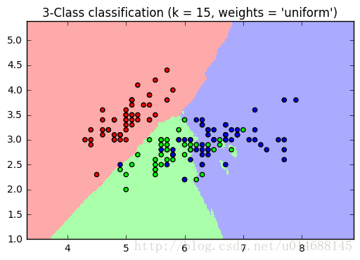
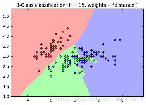
for weights in ['uniform', 'distance']:
# 初始化分类器
clf = neighbors.KNeighborsClassifier(n_neighbors, weights=weights)
# 数据拟合
clf.fit(X, y)
# 生成分类器边界
x_min, x_max = X[:, 0].min() - 1, X[:, 0].max() + 1
y_min, y_max = X[:, 1].min() - 1, X[:, 1].max() + 1
xx, yy = np.meshgrid(np.arange(x_min, x_max, h),
np.arange(y_min, y_max, h))
Z = clf.predict(np.c_[xx.ravel(), yy.ravel()])
Z = Z.reshape(xx.shape)
plt.figure()
plt.pcolormesh(xx, yy, Z, cmap=cmap_light)
# 可视化数据样例
plt.scatter(X[:, 0], X[:, 1], c=y, cmap=cmap_bold)
plt.xlim(xx.min(), xx.max())
plt.ylim(yy.min(), yy.max())
plt.title("3-Class classification (k = %i, weights = '%s')"
% (n_neighbors, weights))
plt.show()可视化如下:
Nearest Neighbors regression
回归使用了KNeighborsRegressor(),表面上就这区别,来看看它的使用,也是so easy。
模拟数据生成
# 1.6.3 Nearest Neighbors Regression

# generate sample data
import numpy as np
import matplotlib.pyplot as plt
from sklearn import neighbors

np.random.seed(0)

X = np.sort(5 * np.random.rand(40, 1), axis=0)
T = np.linspace(0,5,500)[:,np.newaxis]
y = np.sin(X).ravel()

y[::5] += 1 * (0.5-np.random.rand(8))  # 选取下标为 0 ,5,10,...的元素,随机加入噪声
数据预测与可视化
n_neighbors = 5
for i, weights in enumerate(['uniform','distance']):
    knn = neighbors.KNeighborsRegressor(n_neighbors,weights=weights)
    y_ = knn.fit(X,y).predict(T)

    plt.subplot(2,1,i+1)
    plt.scatter(X,y,c='k',label='data')
    plt.plot(T,y_,c='g',label='prediction')
    plt.axis('tight')
    plt.legend()
    plt.title("KNeighborsRegressor (k = %i, weights = '%s')" % (n_neighbors,
                                                                weights))
plt.show()
可视化如下:
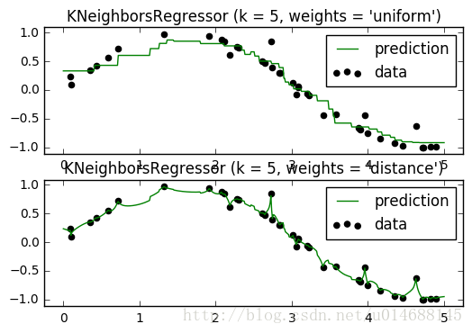
效果还是可以的吧,”distance” 参数对噪声比较敏感,照图的意思是出现了过拟合现象,也不知道实际用knn做回归效果如何。
接下来的官方例子比较有趣,看上去也比较恐怖。给定了一堆人脸图像,现在把图片切分成两半部分,输入=上部分数据,输出=下部分数据。意思就是说根据人的上半脸,可以训练出一个模型来预测下半脸长什么样,我的天。
数据加载与类库导入
import numpy as np
import matplotlib.pyplot as plt

from sklearn.datasets import fetch_olivetti_faces
from sklearn.utils.validation import check_random_state

from sklearn.ensemble import ExtraTreesRegressor
from sklearn.neighbors import KNeighborsRegressor
from sklearn.linear_model import LinearRegression
from sklearn.linear_model import RidgeCV

# load the faces datasets
data = fetch_olivetti_faces()
targets = data.target

# data.images [400,64,64] -> data [400,4096]
data = data.images.reshape(len(data.images),-1)


train = data[targets <30]
test = data[targets >=30]

# 随机选取5张图做测试
n_faces = 5
rng = check_random_state(4)
face_ids = rng.randint(test.shape[0],size=(n_faces,)) # 随机产生大小为size的矩阵【row,col】,范围在[0,test.shape[0])之间
test = test[face_ids,:]

n_pixels = data.shape[1]

# 图的上半部分作为输入向量
X_train = train[:, :np.ceil(0.5 * n_pixels)]  # Upper half of the faces
# 图的下半部分作为输出向量
y_train = train[:, np.floor(0.5 * n_pixels):]  # Lower half of the faces

# 预测输入向量
X_test = test[:, :np.ceil(0.5 * n_pixels)]
# 预测输出向量
y_test = test[:, np.floor(0.5 * n_pixels):]
训练数据并可视化
# 真是个恐怖的实验。。。这些分类器想要根据人脸的上半部分生成人脸的下边部分。

# fit estimators 对比四种分类器分类效果
ESTIMATORS = {
    "Extra trees": ExtraTreesRegressor(n_estimators=10, max_features=32,
                                       random_state=0),
    "K-nn": KNeighborsRegressor(),
    "Linear regression": LinearRegression(),
    "Ridge": RidgeCV(),
}

y_test_predict = dict()

for name,estimator in ESTIMATORS.items():
    estimator.fit(X_train,y_train)
    y_test_predict[name] = estimator.predict(X_test)

# Plot the completed faces
image_shape = (64, 64)

n_cols = 1 + len(ESTIMATORS)
plt.figure(figsize=(2. * n_cols, 2.26 * n_faces))
plt.suptitle("Face completion with multi-output estimators", size=16)

for i in range(n_faces):
    true_face = np.hstack((X_test[i], y_test[i]))

    if i:
        sub = plt.subplot(n_faces, n_cols, i * n_cols + 1)
    else:
        sub = plt.subplot(n_faces, n_cols, i * n_cols + 1,
                          title="true faces")


    sub.axis("off")
    sub.imshow(true_face.reshape(image_shape),
               cmap=plt.cm.gray,
               interpolation="nearest")

    for j, est in enumerate(sorted(ESTIMATORS)):
        completed_face = np.hstack((X_test[i], y_test_predict[est][i]))

        if i:
            sub = plt.subplot(n_faces, n_cols, i * n_cols + 2 + j)

        else:
            sub = plt.subplot(n_faces, n_cols, i * n_cols + 2 + j,
                              title=est)

        sub.axis("off")
        sub.imshow(completed_face.reshape(image_shape),
                   cmap=plt.cm.gray,
                   interpolation="nearest")

plt.show()
可视化如下:
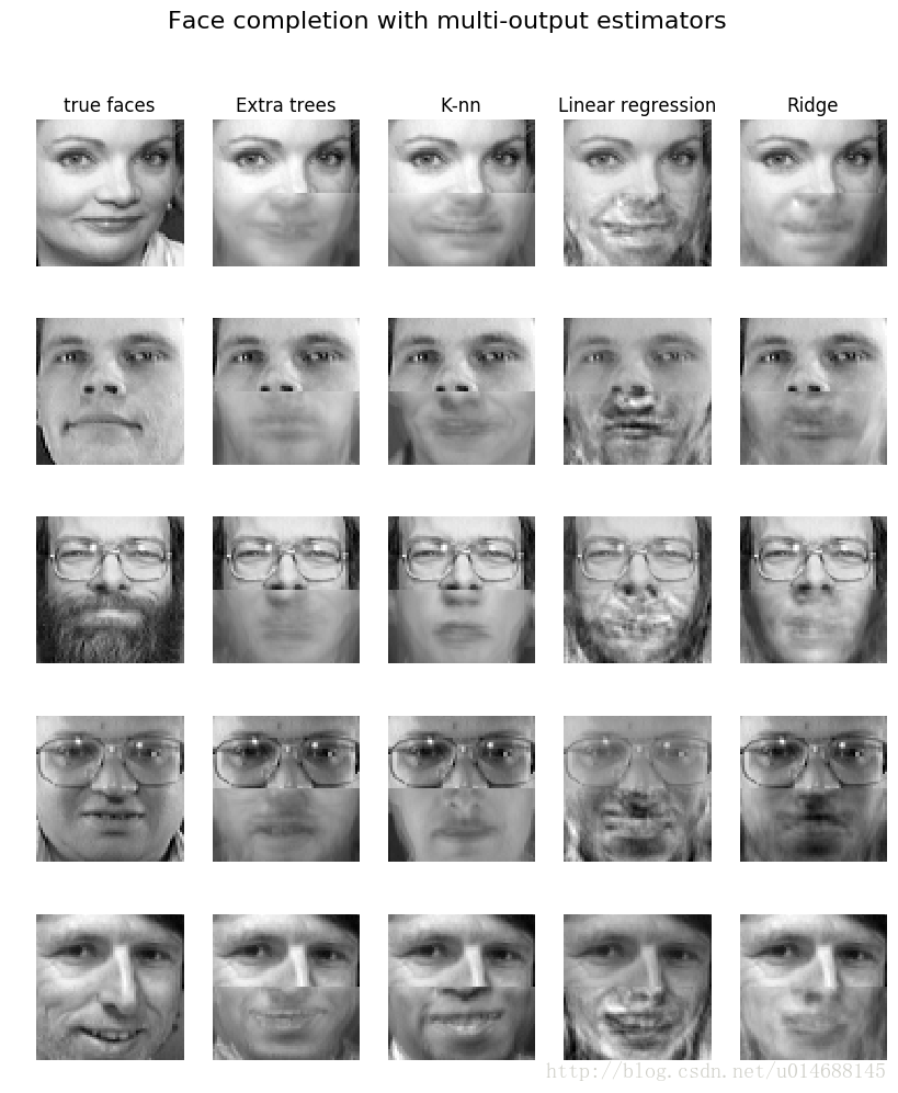
哇,说真的,这些分类器所预测的结果跟真实数据还真的挺神似。这两个案例都使用同样的结构knn = neighbors.KNeighborsRegressor(n_neighbors, weights=weights)和y_ = knn.fit(X, y).predict(T),接下来咱们就进入方法内部一探究竟吧。
源码剖析
在上一篇中,我们总结了数据X到搜索结构映射的调用链,如下所示。
以及k近邻查询的调用链,如下所示:
所以说,非监督的学习由上面两个流程就实现了,由NeighborsBase进行数据X的拟合映射,由KNeighborsMixin负责K近邻的查找。那么现在应该怎么构建监督学习呢?首先它们两者的区别在于:
- 监督学习的
fit()方法和非监督学习的fit()方法不同,一个为fit(X,y),而非监督为fit(X)。 - 非监督学习没有
predict()方法。
但是在这里,我们是否可以让监督学习调用NeighborsBase的fit(X)方法?在k近邻的分类中,是完全可以实现数据X结构映射和predict(y)的分离的。所以一个想法就是增加一个适配器类,让监督学习的fit(X,y) - > fit(X),这样就实现了接口的通用。来看看源码吧!
分类问题
客户端调用
clf = neighbors.KNeighborsClassifier(n_neighbors, weights=weights)
clf.fit(X, y)

clf.predict(X)
clf.score(X)KNeighborsClassifier位于Neighbors包下的classification.py文件下。
class KNeighborsClassifier(NeighborsBase, KNeighborsMixin,
                           SupervisedIntegerMixin, ClassifierMixin):
       def __init__(self, n_neighbors=5,
                 weights='uniform', algorithm='auto', leaf_size=30,
                 p=2, metric='minkowski', metric_params=None, n_jobs=1,
                 **kwargs):

        self._init_params(n_neighbors=n_neighbors,
                          algorithm=algorithm,
                          leaf_size=leaf_size, metric=metric, p=p,
                          metric_params=metric_params, n_jobs=n_jobs, **kwargs)
        self.weights = _check_weights(weights)

    def predict(self, X):
        X = check_array(X, accept_sparse='csr')

        neigh_dist, neigh_ind = self.kneighbors(X)

        classes_ = self.classes_
        _y = self._y
        if not self.outputs_2d_:
            _y = self._y.reshape((-1, 1))
            classes_ = [self.classes_]

        n_outputs = len(classes_)
        n_samples = X.shape[0]
        weights = _get_weights(neigh_dist, self.weights)

        y_pred = np.empty((n_samples, n_outputs), dtype=classes_[0].dtype)
        for k, classes_k in enumerate(classes_):
            if weights is None:
                mode, _ = stats.mode(_y[neigh_ind, k], axis=1)
            else:
                mode, _ = weighted_mode(_y[neigh_ind, k], weights, axis=1)

            mode = np.asarray(mode.ravel(), dtype=np.intp)
            y_pred[:, k] = classes_k.take(mode)

        if not self.outputs_2d_:
            y_pred = y_pred.ravel()

return y_pred 该类的构造方法中的内容和之前分析的一模一样,没什么可以说的,就是交给了父类NeighborsBase做统一的初始化操作。当相比于非监督NearestNeighbors类,多了一个predict(X)方法,这个predict()的位置值得思考,暂且不去分析。
分类器初始化参数后,自然要开始拟合操作了,重点关注它的fit(X,y)操作,它在哪个基类中呢?在他的父类中有个SupervisedIntegerMixin实现了fit(X,y)操作,该基类同样位于base.py中,源码如下:
class SupervisedIntegerMixin(object):
    def fit(self, X, y):

        if not isinstance(X, (KDTree, BallTree)):
            X, y = check_X_y(X, y, "csr", multi_output=True)

        if y.ndim == 1 or y.ndim == 2 and y.shape[1] == 1:
            if y.ndim != 1:
                warnings.warn("A column-vector y was passed when a 1d array "
                              "was expected. Please change the shape of y to "
                              "(n_samples, ), for example using ravel().",
                              DataConversionWarning, stacklevel=2)

            self.outputs_2d_ = False
            y = y.reshape((-1, 1))
        else:
            self.outputs_2d_ = True

        check_classification_targets(y)
        self.classes_ = []
        self._y = np.empty(y.shape, dtype=np.int)
        for k in range(self._y.shape[1]):
            classes, self._y[:, k] = np.unique(y[:, k], return_inverse=True)
            self.classes_.append(classes)

        if not self.outputs_2d_:
            self.classes_ = self.classes_[0]
            self._y = self._y.ravel()
        # 它实质还是调用了NeighborsBase的fit方法
return self._fit(X)从代码可以看出,fit(X,y)实质上还是在调用self._fit(X),而前面的一大堆代码是在做些检查和记录y的值。
现在就剩下predict(X)方法和score(X)方法了,继续KNeighborsClassifier类的分析,它是predict(X)定义的地方,为什么predict(X)不放在某个父类中呢?或许是因为在做预测时,只有两种可能方案,即【回归】和【分类】,而回归和分类这两种方法的predict(X)结构是完全不同的,所以没必要把它们抽象一层放入基类中。
在KNeighborsClassifier中还会继承一个整个sklearn.base下的ClassifierMixin,它是一个给分类器的预测效果进行评分的接口,代码位于sklearn包下的base.py中,如下:
class ClassifierMixin(object):
    """Mixin class for all classifiers in scikit-learn."""
    _estimator_type = "classifier"

    def score(self, X, y, sample_weight=None):
        from .metrics import accuracy_score
        return accuracy_score(y, self.predict(X), sample_weight=sample_weight)
也很简单,因为这个接口各种分类方法的score打分机制是一样的,所以完全可以放在最大的一个基类中,没问题。
来看看整个分类的调用链吧,简单易懂。
回归问题
clf = neighbors.KNeighborsRegressor(n_neighbors, weights=weights)
clf.fit(X, y)

clf.predict(X)
clf.score(X)
回归的结构和分类的结构是完全一模一样,一一对称的,所以我们就不贴代码重复分析了,只是列出它的继承结构和相关类。
KNeighborsRegressor类在Neighbors包下的regression.py中,它同样有四个父类:
- NeighborsBase:参数初始化,fit(X)的调度。
- KNeighborsMixin:k近邻的查询。
- SupervisedFloatMixin:适配器,fit(X,y)到fit(x)的适配。
- RegressorMixin:回归打分机制。
同样的,它有如下调用链。
Ok,整个Neighbors系列的架构算是分析完毕了,没什么特别指出的地方,框架有了,没啥内容,后续将着重算法ball_tree和kd_tree性能对比,来点干货,敬请期待。
最后
以上就是重要夏天最近收集整理的关于sklearn 源码分析系列:neighbors(3) sklearn 源码分析系列:neighbors(3) 的全部内容,更多相关sklearn内容请搜索靠谱客的其他文章。


发表评论 取消回复