一、实现卷积-池化-激活

1. Numpy版本：手工实现 卷积-池化-激活

自定义卷积算子、池化算子实现，我们通过老师给的代码，添加注释，便于自己和别人理解。
代码如下：

import numpy as np
#初始化一张X图片矩阵
x = np.array([[-1, -1, -1, -1, -1, -1, -1, -1, -1],
              [-1, 1, -1, -1, -1, -1, -1, 1, -1],
              [-1, -1, 1, -1, -1, -1, 1, -1, -1],
              [-1, -1, -1, 1, -1, 1, -1, -1, -1],
              [-1, -1, -1, -1, 1, -1, -1, -1, -1],
              [-1, -1, -1, 1, -1, 1, -1, -1, -1],
              [-1, -1, 1, -1, -1, -1, 1, -1, -1],
              [-1, 1, -1, -1, -1, -1, -1, 1, -1],
              [-1, -1, -1, -1, -1, -1, -1, -1, -1]])
#输出原矩阵
print("x=n", x)
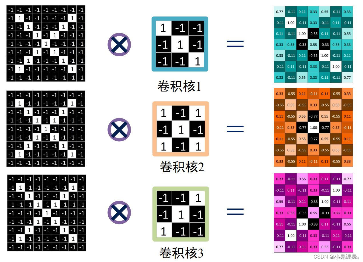
# 初始化 三个 卷积核
Kernel = [[0 for i in range(0, 3)] for j in range(0, 3)]
#参考图卷积核1
Kernel[0] = np.array([[1, -1, -1],
                      [-1, 1, -1],
                      [-1, -1, 1]])
#参考图卷积核2
Kernel[1] = np.array([[1, -1, 1],
                      [-1, 1, -1],
                      [1, -1, 1]])
#参考图卷积核3
Kernel[2] = np.array([[-1, -1, 1],
                      [-1, 1, -1],
                      [1, -1, -1]])
 
# --------------- 卷积  ---------------
stride = 1  # 步长
feature_map_h = 7  # 特征图的高
feature_map_w = 7  # 特征图的宽
feature_map = [0 for i in range(0, 3)]  # 初始化3个特征图
for i in range(0, 3):
    feature_map[i] = np.zeros((feature_map_h, feature_map_w))  # 初始化特征图
for h in range(feature_map_h):        # 向下滑动，得到卷积后的固定行
    for w in range(feature_map_w):  # 向右滑动，得到卷积后的固定行的列
        v_start = h * stride  # 滑动窗口的起始行（高）
        v_end = v_start + 3  # 滑动窗口的结束行（高）
        h_start = w * stride  # 滑动窗口的起始列（宽）
        h_end = h_start + 3  # 滑动窗口的结束列（宽）
        window = x[v_start:v_end, h_start:h_end]  # 从图切出一个滑动窗口
        for i in range(0, 3):
            feature_map[i][h, w] = np.divide(np.sum(np.multiply(window, Kernel[i][:, :])), 9)
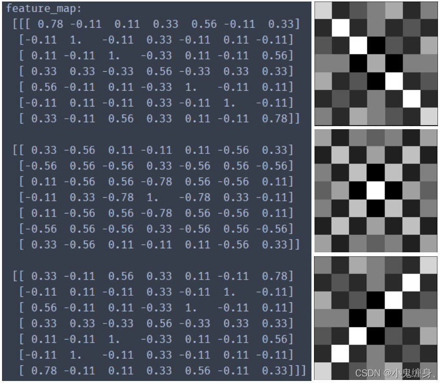
print("feature_map:n", np.around(feature_map, decimals=2))
 
# --------------- 池化  ---------------
pooling_stride = 2  # 步长
pooling_h = 4  # 特征图的高
pooling_w = 4  # 特征图的宽
feature_map_pad_0 = [[0 for i in range(0, 8)] for j in range(0, 8)]
for i in range(0, 3):  # 特征图 补 0 ，行 列 都要加 1 (因为上一层是奇数，池化窗口用的偶数)
    feature_map_pad_0[i] = np.pad(feature_map[i], ((0, 1), (0, 1)), 'constant', constant_values=(0, 0))
# print("feature_map_pad_0 0:n", np.around(feature_map_pad_0[0], decimals=2))
 
pooling = [0 for i in range(0, 3)]
for i in range(0, 3):
    pooling[i] = np.zeros((pooling_h, pooling_w))  # 初始化特征图
for h in range(pooling_h):  # 向下滑动，得到卷积后的固定行
    for w in range(pooling_w):  # 向右滑动，得到卷积后的固定行的列
        v_start = h * pooling_stride  # 滑动窗口的起始行（高）
        v_end = v_start + 2  # 滑动窗口的结束行（高）
        h_start = w * pooling_stride  # 滑动窗口的起始列（宽）
        h_end = h_start + 2  # 滑动窗口的结束列（宽）
        for i in range(0, 3):
            pooling[i][h, w] = np.max(feature_map_pad_0[i][v_start:v_end, h_start:h_end])
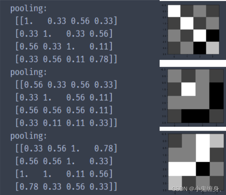
print("pooling:n", np.around(pooling[0], decimals=2))
print("pooling:n", np.around(pooling[1], decimals=2))
print("pooling:n", np.around(pooling[2], decimals=2))
 

# --------------- 激活  ---------------
def relu(x):
    return (abs(x) + x) / 2
 

relu_map_h = 7  # 特征图的高
relu_map_w = 7  # 特征图的宽
relu_map = [0 for i in range(0, 3)]  # 初始化3个特征图
for i in range(0, 3):
    relu_map[i] = np.zeros((relu_map_h, relu_map_w))  # 初始化特征图

for i in range(0, 3):
    relu_map[i] = relu(feature_map[i])

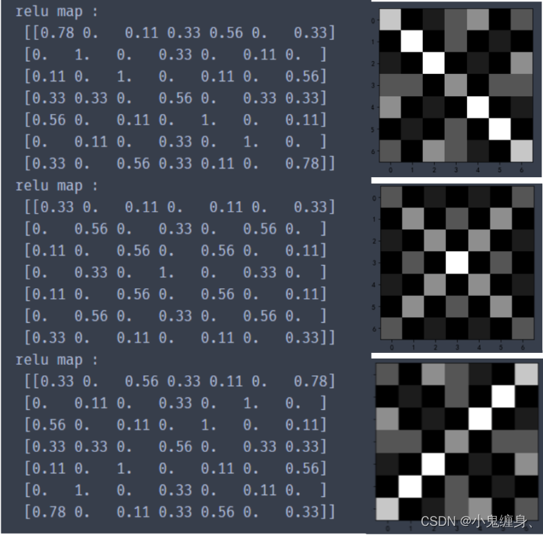
print("relu map :n",np.around(relu_map[0], decimals=2))
print("relu map :n",np.around(relu_map[1], decimals=2))
print("relu map :n",np.around(relu_map[2], decimals=2))

三个卷积核卷积结果：

三个池化层的结果：

激活层后三个特征图的结果：

2. Pytorch版本：调用函数实现 卷积-池化-激活

调用框架自带算子实现，对比自定义算子。
代码实现：

# https://blog.csdn.net/qq_26369907/article/details/88366147
# https://zhuanlan.zhihu.com/p/405242579
import numpy as np
import torch
import torch.nn as nn
 
x = torch.tensor([[[[-1, -1, -1, -1, -1, -1, -1, -1, -1],
                    [-1, 1, -1, -1, -1, -1, -1, 1, -1],
                    [-1, -1, 1, -1, -1, -1, 1, -1, -1],
                    [-1, -1, -1, 1, -1, 1, -1, -1, -1],
                    [-1, -1, -1, -1, 1, -1, -1, -1, -1],
                    [-1, -1, -1, 1, -1, 1, -1, -1, -1],
                    [-1, -1, 1, -1, -1, -1, 1, -1, -1],
                    [-1, 1, -1, -1, -1, -1, -1, 1, -1],
                    [-1, -1, -1, -1, -1, -1, -1, -1, -1]]]], dtype=torch.float)
print(x.shape)
print(x)
 
print("--------------- 卷积  ---------------")
conv1 = nn.Conv2d(1, 1, (3, 3), 1)  # in_channel , out_channel , kennel_size , stride
conv1.weight.data = torch.Tensor([[[[1, -1, -1],
                                    [-1, 1, -1],
                                    [-1, -1, 1]]
                                   ]])
conv2 = nn.Conv2d(1, 1, (3, 3), 1)  # in_channel , out_channel , kennel_size , stride
conv2.weight.data = torch.Tensor([[[[1, -1, 1],
                                    [-1, 1, -1],
                                    [1, -1, 1]]
                                   ]])
conv3 = nn.Conv2d(1, 1, (3, 3), 1)  # in_channel , out_channel , kennel_size , stride
conv3.weight.data = torch.Tensor([[[[-1, -1, 1],
                                    [-1, 1, -1],
                                    [1, -1, -1]]
                                   ]])
 
feature_map1 = conv1(x)
feature_map2 = conv2(x)
feature_map3 = conv3(x)
 
print(feature_map1 / 9)
print(feature_map2 / 9)
print(feature_map3 / 9)
# img = torch.tensor(feature_map3).data.squeeze().numpy()  # 将输出转换为图片的格式
# plt.imshow(img, cmap='gray')
print("--------------- 池化  ---------------")
max_pool = nn.MaxPool2d(2, padding=0, stride=2)  # Pooling
zeroPad = nn.ZeroPad2d(padding=(0, 1, 0, 1))  # pad 0 , Left Right Up Down
 
feature_map_pad_0_1 = zeroPad(feature_map1)
feature_pool_1 = max_pool(feature_map_pad_0_1)
feature_map_pad_0_2 = zeroPad(feature_map2)
feature_pool_2 = max_pool(feature_map_pad_0_2)
feature_map_pad_0_3 = zeroPad(feature_map3)
feature_pool_3 = max_pool(feature_map_pad_0_3)
 
print(feature_pool_1.size())
print(feature_pool_1 / 9)
print(feature_pool_2 / 9)
print(feature_pool_3 / 9)
 
print("--------------- 激活  ---------------")
activation_function = nn.ReLU()
 
feature_relu1 = activation_function(feature_map1)
feature_relu2 = activation_function(feature_map2)
feature_relu3 = activation_function(feature_map3)
print(feature_relu1 / 9)
print(feature_relu2 / 9)
print(feature_relu3 / 9)
 

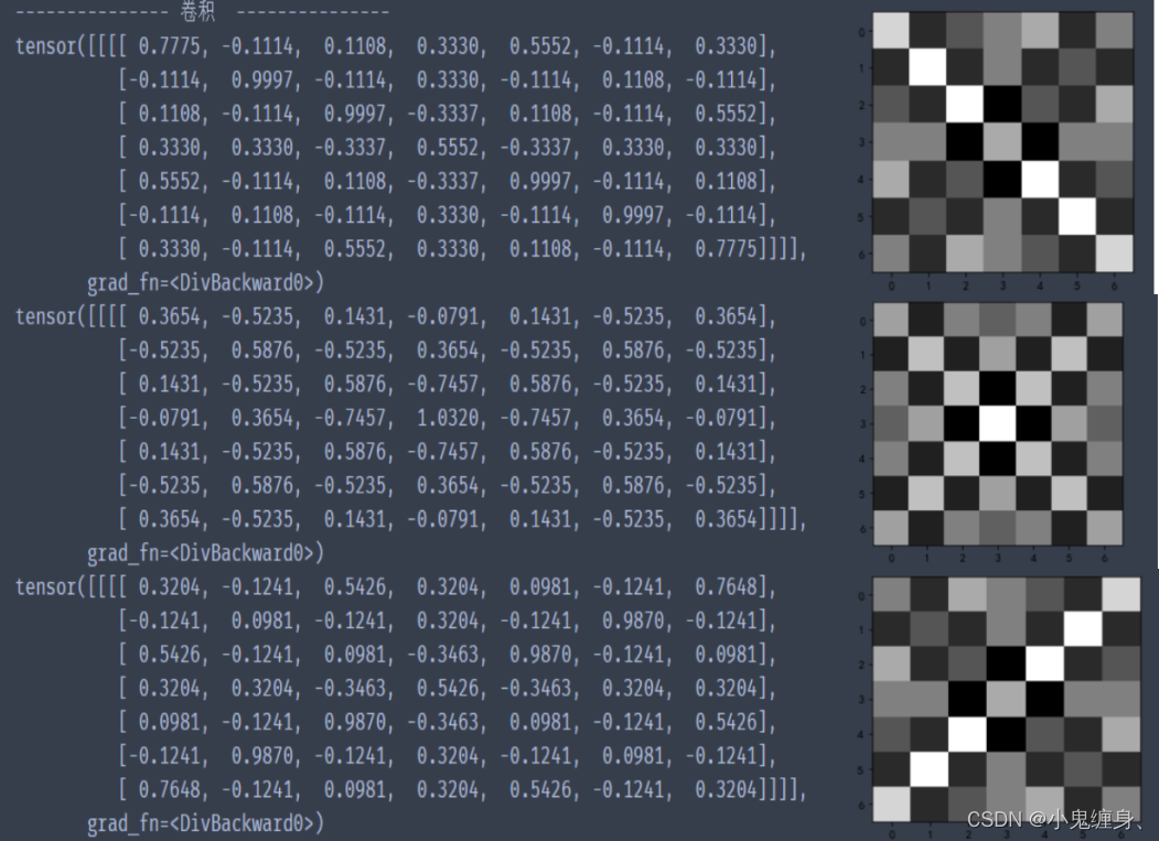
三层卷积结果：

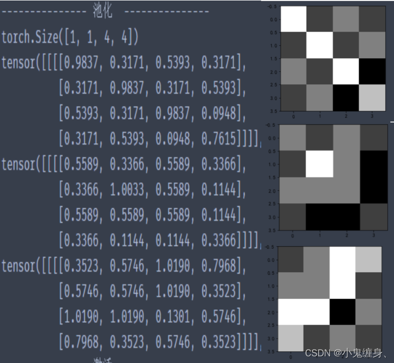
池化后的结果：

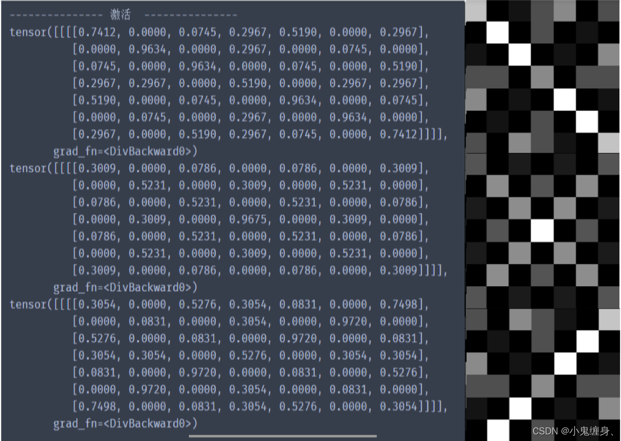
激活层之后：

对比自定义算子

卷积层对比，发现两者基本没有区别。

池化层对比，两者基本上并无差别。

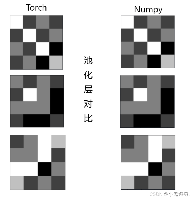
激活层对比：

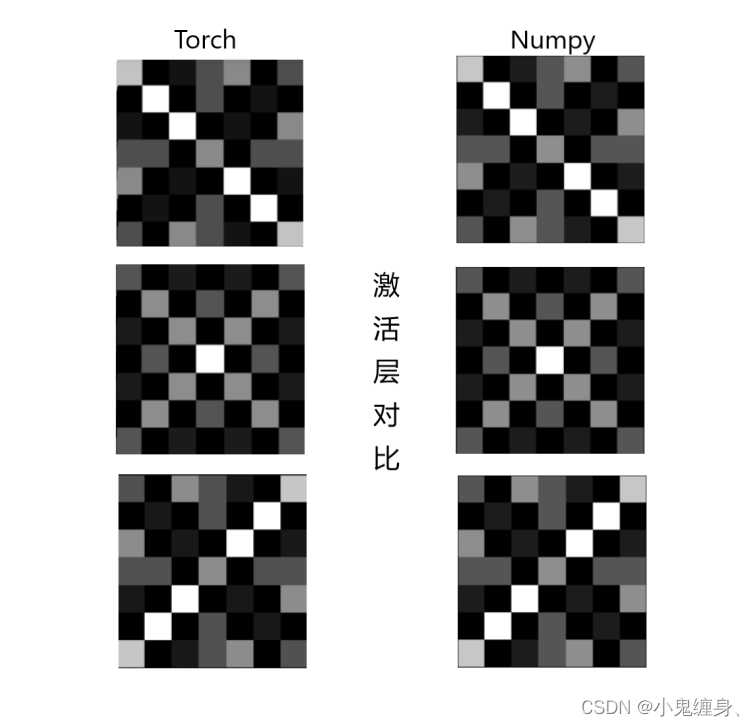
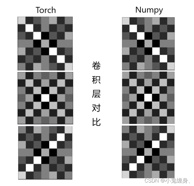
结果：
可见，在可视化两者对比上，torch和numpy并无差别，但是对于自定义算子和torch相比，Torch的输出相对于自定义算子来说表现的更加精确。

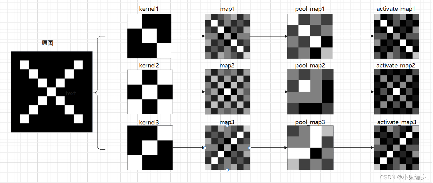
3. 可视化：了解数字与图像之间的关系

可视化卷积核和特征图。
制图如下：

二、 基于CNN的XO识别

1. 数据集

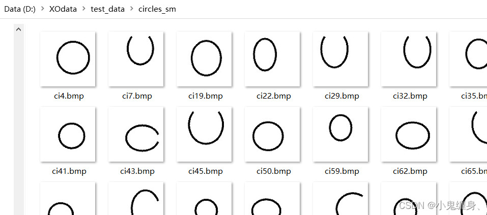
1.1 数据集展示：

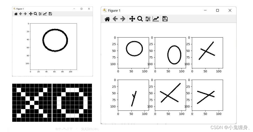
'O’数据集：

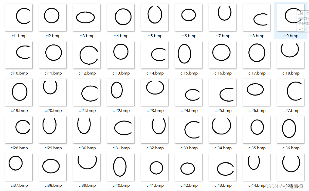
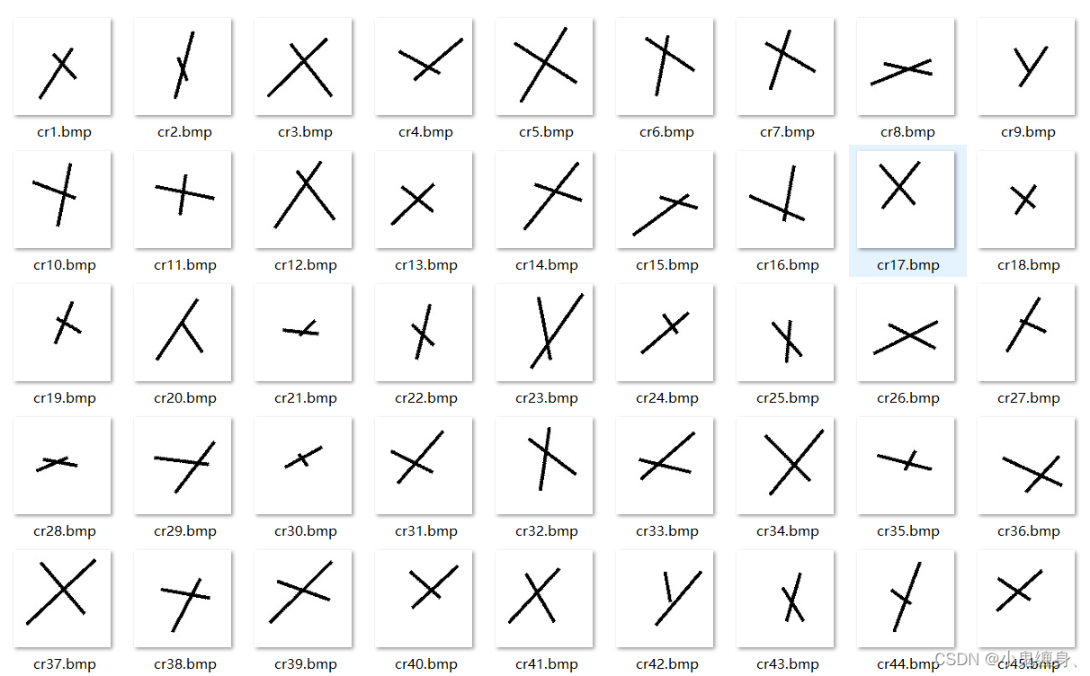
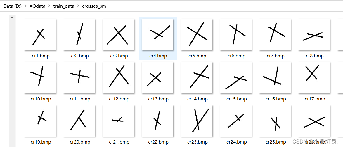
'X’数据集：

1.2 划分训练集和测试集

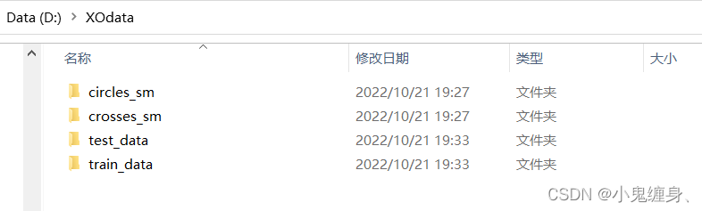
如何将这两个文件夹分为训练集和测试集呢？我将这两个文件夹放在了：D:XOdata中，用代码分隔开来。
共2000张图片，X、O各1000张。
从X、O文件夹，这里我们取出200作为测试集。
文件夹D:XOdatatrain_data：放置训练集 1600张图片
文件夹D:XOdatatest_data： 放置测试集 400张图片

分离训练集和测试集代码如下：

#
import os
import random
import shutil
from shutil import copy2

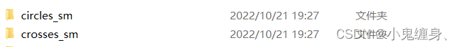
datadir_normal = "D:\XOdata\crosses_sm"

all_data = os.listdir(datadir_normal)  # （图片文件夹）
num_all_data = len(all_data)
print("num_all_data: " + str(num_all_data))
index_list = list(range(num_all_data))

random.shuffle(index_list)
num = 0

trainDir =  "D:\XOdata\train_data\crosses_sm"  # （将训练集放在这个文件夹下）
if not os.path.exists(trainDir):
    os.makedirs(trainDir)

testDir = "D:\XOdata\test_data\crosses_sm"  # （将测试集放在这个文件夹下）
if not os.path.exists(testDir):
    os.makedirs(testDir)

for i in index_list:
    fileName = os.path.join(datadir_normal, all_data[i])
    if num < num_all_data * 0.8:
        copy2(fileName, trainDir)
    else:
        copy2(fileName, testDir)
    num += 1

print(len(trainDir))
print(len(testDir))

分离结果：

2. 构建模型

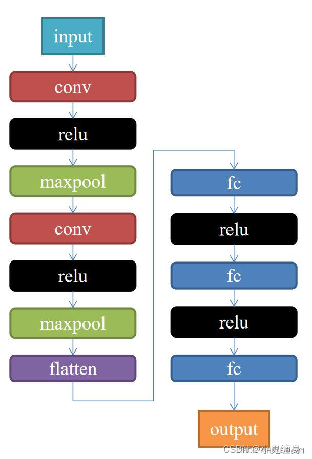
下面我们根据上图构建网络，代码如下：

import torch.nn as nn
import torch
class Net(nn.Module):
    def __init__(self):
        super(Net, self).__init__()
        self.conv1 = nn.Conv2d(1, 9, 3)
        self.maxpool = nn.MaxPool2d(2, 2)
        self.conv2 = nn.Conv2d(9, 5, 3)

        self.relu = nn.ReLU()
        self.fc1 = nn.Linear(27 * 27 * 5, 1200)
        self.fc2 = nn.Linear(1200, 64)
        self.fc3 = nn.Linear(64, 2)

    def forward(self, x):
        x = self.maxpool(self.relu(self.conv1(x)))
        x = self.maxpool(self.relu(self.conv2(x)))
        x = x.view(-1, 27 * 27 * 5)
        x = self.relu(self.fc1(x))
        x = self.relu(self.fc2(x))
        x = self.fc3(x)
        return x

3. 训练模型

import torch
from torchvision import transforms, datasets
import torch.nn as nn
from torch.utils.data import DataLoader
import matplotlib.pyplot as plt
import torch.optim as optim
 
transforms = transforms.Compose([
    transforms.ToTensor(),  # 把图片进行归一化，并把数据转换成Tensor类型
    transforms.Grayscale(1)  # 把图片 转为灰度图
])
 
path = r'D:XOdatatrain_data'
path_test = r'D:XOdatatest_data'

data_train = datasets.ImageFolder(path, transform=transforms)
data_test = datasets.ImageFolder(path_test, transform=transforms)
 
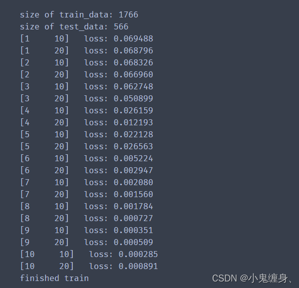
print("size of train_data:",len(data_train))
print("size of test_data:",len(data_test))
 
data_loader = DataLoader(data_train, batch_size=64, shuffle=True)
data_loader_test = DataLoader(data_test, batch_size=64, shuffle=True)
model = Net()
 
criterion = torch.nn.CrossEntropyLoss()  # 损失函数 交叉熵损失函数
optimizer = torch.optim.SGD(model.parameters(), lr=0.1)  # 优化函数：随机梯度下降
 
epochs = 10
for epoch in range(epochs):
    running_loss = 0.0
    for i, data in enumerate(data_loader):
        images, label = data
        out = model(images)
        loss = criterion(out, label)

        optimizer.zero_grad()
        loss.backward()
        optimizer.step()

        running_loss += loss.item()
        if (i + 1) % 10 == 0:
            print('[%d  %5d]   loss: %.6f' % (epoch + 1, i + 1, running_loss / 100))
            running_loss = 0.0

print('finished train')
 
# 保存模型
torch.save(model, 'model_name.pth')  # 保存的是模型， 不止是w和b权重值

训练结果：

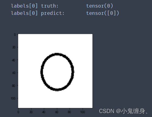
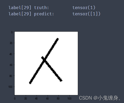
4. 测试训练好的模型

# 读取模型
model_load = torch.load('model_name.pth')
# 读取一张图片 images[0]，测试
print("label[0] truth:t", label[0])
x = images[0]
x = x.reshape([1,1,116,116])
predicted = torch.max(model_load(x), 1)
print("label[0] predict:t", predicted.indices)
 
img = images[0].data.squeeze().numpy()  # 将输出转换为图片的格式
plt.imshow(img, cmap='gray')
plt.show()

测试结果：

5. 计算模型的准确率

# 读取模型
model_load = Net()
model_load.load_state_dict(torch.load('model_name.pth'))
correct = 0
total = 0
with torch.no_grad():  # 进行评测的时候网络不更新梯度
    for data in data_loader_test:  # 读取测试集
        images, labels = data
        outputs = model_load(images)
        _, predicted = torch.max(outputs.data, 1)  # 取出 最大值的索引 作为 分类结果
        total += labels.size(0)  # labels 的长度
        correct += (predicted == labels).sum().item()  # 预测正确的数目
print('Accuracy of the network on the  test images: %f %%' % (100. * correct / total))

准确率：

Accuracy of the network on the test images: 100.000000 %

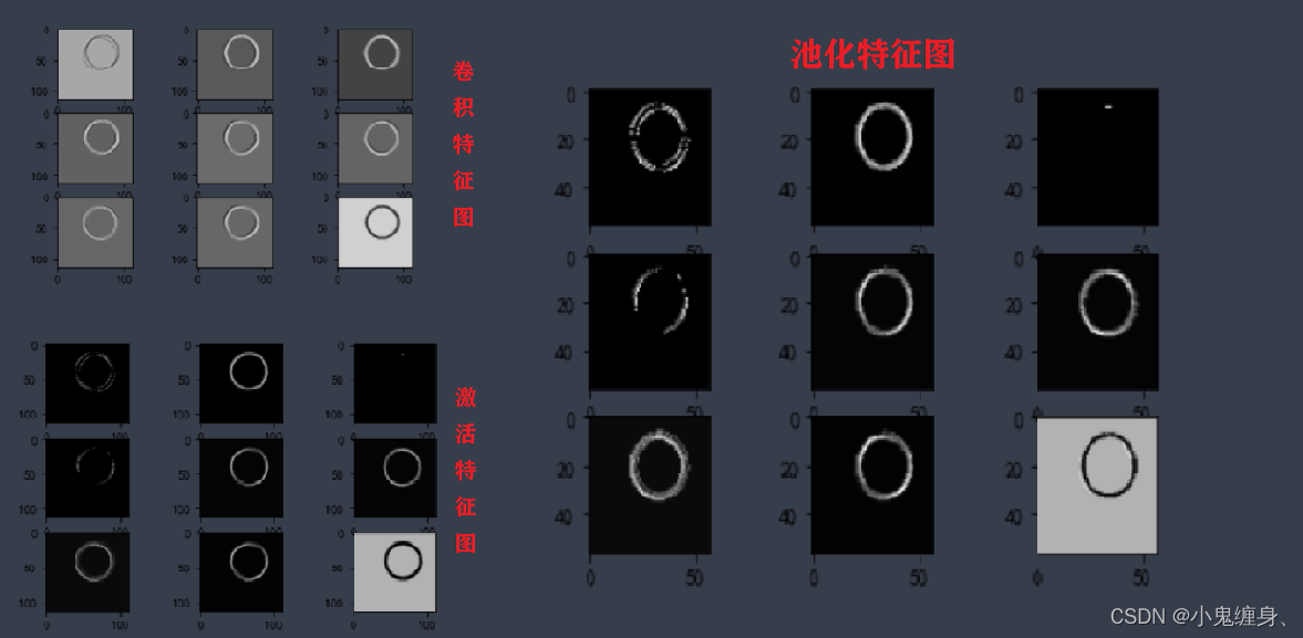
6. 查看训练好的模型的特征图

代码：

# 看看每层的 卷积核 长相，特征图 长相
# 获取网络结构的特征矩阵并可视化
import torch
import matplotlib.pyplot as plt
import numpy as np
from PIL import Image
from torchvision import transforms, datasets
import torch.nn as nn
from torch.utils.data import DataLoader
 
#  定义图像预处理过程(要与网络模型训练过程中的预处理过程一致)
 
transforms = transforms.Compose([
    transforms.ToTensor(),  # 把图片进行归一化，并把数据转换成Tensor类型
    transforms.Grayscale(1)  # 把图片 转为灰度图
])
path = r'D:XOdatatrain_data'
data_train = datasets.ImageFolder(path, transform=transforms)
data_loader = DataLoader(data_train, batch_size=64, shuffle=True)
for i, data in enumerate(data_loader):
    images, labels = data
    print(images.shape)
    print(labels.shape)
    break


class Net(nn.Module):
    def __init__(self):
        super(Net, self).__init__()
        self.conv1 = nn.Conv2d(1, 9, 3)  # in_channel , out_channel , kennel_size , stride
        self.maxpool = nn.MaxPool2d(2, 2)
        self.conv2 = nn.Conv2d(9, 5, 3)  # in_channel , out_channel , kennel_size , stride

        self.relu = nn.ReLU()
        self.fc1 = nn.Linear(27 * 27 * 5, 1200)  # full connect 1
        self.fc2 = nn.Linear(1200, 64)  # full connect 2
        self.fc3 = nn.Linear(64, 2)  # full connect 3

    def forward(self, x):
        outputs = []
        x = self.conv1(x)
        outputs.append(x)
        x = self.relu(x)
        outputs.append(x)
        x = self.maxpool(x)
        outputs.append(x)
        x = self.conv2(x)

        x = self.relu(x)

        x = self.maxpool(x)

        x = x.view(-1, 27 * 27 * 5)
        x = self.relu(self.fc1(x))
        x = self.relu(self.fc2(x))
        x = self.fc3(x)
        return outputs


# create model
model1 = Net()
 
# load model weights加载预训练权重
# model_weight_path ="./AlexNet.pth"
model_weight_path = "model_name.pth"
model1.load_state_dict(torch.load(model_weight_path))
 
# 打印出模型的结构

print(model1)
 
x = images[0]
x = x.reshape([1,1,116,116])
# forward正向传播过程
out_put = model1(x)
for feature_map in out_put:
    # [N, C, H, W] -> [C, H, W]    维度变换
    im = np.squeeze(feature_map.detach().numpy())
    # [C, H, W] -> [H, W, C]
    im = np.transpose(im, [1, 2, 0])
    print(im.shape)

    # show 9 feature maps
    plt.figure()
    for i in range(9):
        ax = plt.subplot(3, 3, i + 1)  # 参数意义：3：图片绘制行数，5：绘制图片列数，i+1：图的索引
        # [H, W, C]
        # 特征矩阵每一个channel对应的是一个二维的特征矩阵，就像灰度图像一样，channel=1
        # plt.imshow(im[:, :, i])
        plt.imshow(im[:, :, i], cmap='gray')
    plt.show()

输出结果：

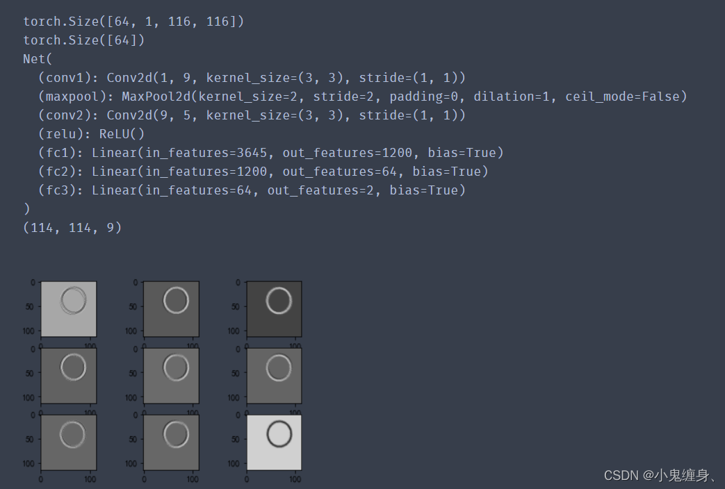
查看训练好的模型的特征图：

7. 查看训练好的模型的卷积核

# 看看每层的 卷积核 长相，特征图 长相
# 获取网络结构的特征矩阵并可视化
import torch
import matplotlib.pyplot as plt
import numpy as np
from PIL import Image
from torchvision import transforms, datasets
import torch.nn as nn
from torch.utils.data import DataLoader
 
plt.rcParams['font.sans-serif'] = ['SimHei']  # 用来正常显示中文标签
plt.rcParams['axes.unicode_minus'] = False  # 用来正常显示负号 #有中文出现的情况，需要u'内容
#  定义图像预处理过程(要与网络模型训练过程中的预处理过程一致)
transforms = transforms.Compose([
    transforms.ToTensor(),  # 把图片进行归一化，并把数据转换成Tensor类型
    transforms.Grayscale(1)  # 把图片 转为灰度图
])
path = r'D:XOdatatrain_data'
data_train = datasets.ImageFolder(path, transform=transforms)
data_loader = DataLoader(data_train, batch_size=64, shuffle=True)
for i, data in enumerate(data_loader):
    images, labels = data
    # print(images.shape)
    # print(labels.shape)
    break


class Net(nn.Module):
    def __init__(self):
        super(Net, self).__init__()
        self.conv1 = nn.Conv2d(1, 9, 3)  # in_channel , out_channel , kennel_size , stride
        self.maxpool = nn.MaxPool2d(2, 2)
        self.conv2 = nn.Conv2d(9, 5, 3)  # in_channel , out_channel , kennel_size , stride

        self.relu = nn.ReLU()
        self.fc1 = nn.Linear(27 * 27 * 5, 1200)  # full connect 1
        self.fc2 = nn.Linear(1200, 64)  # full connect 2
        self.fc3 = nn.Linear(64, 2)  # full connect 3

    def forward(self, x):
        outputs = []
        x = self.maxpool(self.relu(self.conv1(x)))
        # outputs.append(x)
        x = self.maxpool(self.relu(self.conv2(x)))
        outputs.append(x)
        x = x.view(-1, 27 * 27 * 5)
        x = self.relu(self.fc1(x))
        x = self.relu(self.fc2(x))
        x = self.fc3(x)
        return outputs

# create model
model1 = Net()
 
# load model weights加载预训练权重
model_weight_path = "model_name.pth"
model1.load_state_dict(torch.load(model_weight_path))
 
x = images[0]
x = x.reshape([1,1,116,116])
# forward正向传播过程
out_put = model1(x)
 
weights_keys = model1.state_dict().keys()
for key in weights_keys:
    print("key :", key)
    # 卷积核通道排列顺序 [kernel_number, kernel_channel, kernel_height, kernel_width]
    if key == "conv1.weight":
        weight_t = model1.state_dict()[key].numpy()
        print("weight_t.shape", weight_t.shape)
        k = weight_t[:, 0, :, :]  # 获取第一个卷积核的信息参数
        # show 9 kernel ,1 channel
        plt.figure()

        for i in range(9):
            ax = plt.subplot(3, 3, i + 1)  # 参数意义：3：图片绘制行数，5：绘制图片列数，i+1：图的索引
            plt.imshow(k[i, :, :], cmap='gray')
            title_name = 'kernel' + str(i) + ',channel1'
            plt.title(title_name)
        plt.show()

    if key == "conv2.weight":
        weight_t = model1.state_dict()[key].numpy()
        print("weight_t.shape", weight_t.shape)
        k = weight_t[:, :, :, :]  # 获取第一个卷积核的信息参数
        print(k.shape)
        print(k)

        plt.figure()
        for c in range(9):
            channel = k[:, c, :, :]
            for i in range(5):
                ax = plt.subplot(2, 3, i + 1)  # 参数意义：3：图片绘制行数，5：绘制图片列数，i+1：图的索引
                plt.imshow(channel[i, :, :], cmap='gray')
                title_name = 'kernel' + str(i) + ',channel' + str(c)
                plt.title(title_name)
            plt.show()

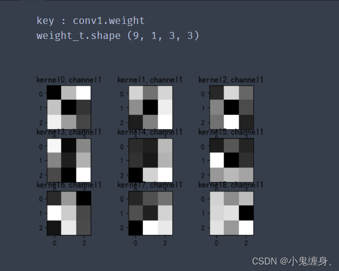
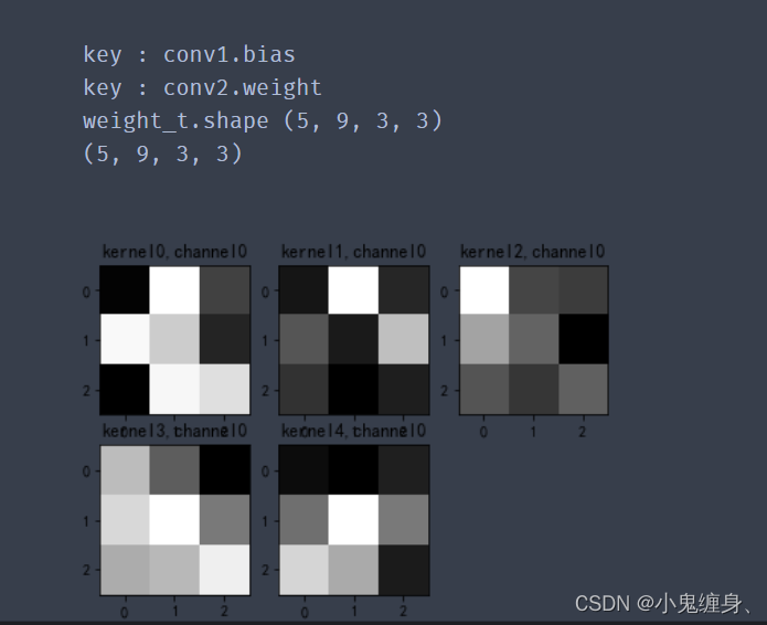
输出结果：
下图中的九个图片是第一轮9个(单通道)的卷积核，CNN的卷积核是模型自己训练得到的，不需要人工干预，类似于FNN中的权值w，通过反向传播，梯度下降不断更新。

第二层卷积：

8. 训练模型源代码

# https://blog.csdn.net/qq_53345829/article/details/124308515
import torch
from torchvision import transforms, datasets
import torch.nn as nn
from torch.utils.data import DataLoader
import matplotlib.pyplot as plt
import torch.optim as optim
 
transforms = transforms.Compose([
    transforms.ToTensor(),  # 把图片进行归一化，并把数据转换成Tensor类型
    transforms.Grayscale(1)  # 把图片 转为灰度图
])
 
path = r'D:XOdatatrain_data'
path_test = r'D:XOdatatest_data'
 
data_train = datasets.ImageFolder(path, transform=transforms)
data_test = datasets.ImageFolder(path_test, transform=transforms)
 
print("size of train_data:",len(data_train))
print("size of test_data:",len(data_test))
 
data_loader = DataLoader(data_train, batch_size=64, shuffle=True)
data_loader_test = DataLoader(data_test, batch_size=64, shuffle=True)
 
for i, data in enumerate(data_loader):
    images, labels = data
    print(images.shape)
    print(labels.shape)
    break

for i, data in enumerate(data_loader_test):
    images, labels = data
    print(images.shape)
    print(labels.shape)
    break


class Net(nn.Module):
    def __init__(self):
        super(Net, self).__init__()
        self.conv1 = nn.Conv2d(1, 9, 3)  # in_channel , out_channel , kennel_size , stride
        self.maxpool = nn.MaxPool2d(2, 2)
        self.conv2 = nn.Conv2d(9, 5, 3)  # in_channel , out_channel , kennel_size , stride

        self.relu = nn.ReLU()
        self.fc1 = nn.Linear(27 * 27 * 5, 1200)  # full connect 1
        self.fc2 = nn.Linear(1200, 64)  # full connect 2
        self.fc3 = nn.Linear(64, 2)  # full connect 3

    def forward(self, x):
        x = self.maxpool(self.relu(self.conv1(x)))
        x = self.maxpool(self.relu(self.conv2(x)))
        x = x.view(-1, 27 * 27 * 5)
        x = self.relu(self.fc1(x))
        x = self.relu(self.fc2(x))
        x = self.fc3(x)
        return x


model = Net()
 
criterion = torch.nn.CrossEntropyLoss()  # 损失函数 交叉熵损失函数
optimizer = optim.SGD(model.parameters(), lr=0.1)  # 优化函数：随机梯度下降
 
epochs = 10
for epoch in range(epochs):
    running_loss = 0.0
    for i, data in enumerate(data_loader):
        images, label = data
        out = model(images)
        loss = criterion(out, label)

        optimizer.zero_grad()
        loss.backward()
        optimizer.step()

        running_loss += loss.item()
        if (i + 1) % 10 == 0:
            print('[%d  %5d]   loss: %.3f' % (epoch + 1, i + 1, running_loss / 100))
            running_loss = 0.0

print('finished train')
 
# 保存模型 torch.save(model.state_dict(), model_path)
torch.save(model.state_dict(), 'model_name1.pth')  # 保存的是模型， 不止是w和b权重值
 
# 读取模型
model = torch.load('model_name1.pth')

9. 测试模型源代码

# https://blog.csdn.net/qq_53345829/article/details/124308515
import torch
from torchvision import transforms, datasets
import torch.nn as nn
from torch.utils.data import DataLoader
import matplotlib.pyplot as plt
import torch.optim as optim
 
transforms = transforms.Compose([
    transforms.ToTensor(),  # 把图片进行归一化，并把数据转换成Tensor类型
    transforms.Grayscale(1)  # 把图片 转为灰度图
])
 
path = r'D:XOdatatrain_data'
path_test = r'D:XOdatatest_data'
 
data_train = datasets.ImageFolder(path, transform=transforms)
data_test = datasets.ImageFolder(path_test, transform=transforms)
 
print("size of train_data:", len(data_train))
print("size of test_data:", len(data_test))
 
data_loader = DataLoader(data_train, batch_size=64, shuffle=True)
data_loader_test = DataLoader(data_test, batch_size=64, shuffle=True)
print(len(data_loader))
print(len(data_loader_test))


class Net(nn.Module):
    def __init__(self):
        super(Net, self).__init__()
        self.conv1 = nn.Conv2d(1, 9, 3)  # in_channel , out_channel , kennel_size , stride
        self.maxpool = nn.MaxPool2d(2, 2)
        self.conv2 = nn.Conv2d(9, 5, 3)  # in_channel , out_channel , kennel_size , stride

        self.relu = nn.ReLU()
        self.fc1 = nn.Linear(27 * 27 * 5, 1200)  # full connect 1
        self.fc2 = nn.Linear(1200, 64)  # full connect 2
        self.fc3 = nn.Linear(64, 2)  # full connect 3

    def forward(self, x):
        x = self.maxpool(self.relu(self.conv1(x)))
        x = self.maxpool(self.relu(self.conv2(x)))
        x = x.view(-1, 27 * 27 * 5)
        x = self.relu(self.fc1(x))
        x = self.relu(self.fc2(x))
        x = self.fc3(x)
        return x

# 读取模型
model = Net()
model.load_state_dict(torch.load('model_name1.pth', map_location='cpu')) # 导入网络的参数
 
# model_load = torch.load('model_name1.pth')
# https://blog.csdn.net/qq_41360787/article/details/104332706
 
correct = 0
total = 0
with torch.no_grad():  # 进行评测的时候网络不更新梯度
    for data in data_loader_test:  # 读取测试集
        images, labels = data
        outputs = model(images)
        _, predicted = torch.max(outputs.data, 1)  # 取出 最大值的索引 作为 分类结果
        total += labels.size(0)  # labels 的长度
        correct += (predicted == labels).sum().item()  # 预测正确的数目
print('Accuracy of the network on the  test images: %f %%' % (100. * correct / total))
 
#  "_," 的解释 https://blog.csdn.net/weixin_48249563/article/details/111387501

参考代码

【2021-2022 春学期】人工智能-作业6：CNN实现XO识别

总结

这次呢，我们实现了一个简单的图片数据集的识别，中间提取并可视化了一些个训练过程，对于其过程训练中的内容更加清楚，感觉还是要跑一下大规模的数据集，但是我尝试了一下那个mnist，感觉mnist六万张图片也不是特别大啊，显示图片就给我卡的要死，可能是自己的电脑配置太拉了，我要吐槽一下，不用说跑大数据集了，就连画图3D粘上去五六张图片就能给我卡死，等到有更好的配置再做一下大的数据集吧。最后就是，这次作业emmm确实挺好的，我也画了好多图来让自己更好的理解和对比，也方便大家理解和比较，如果有错的地方，希望给我指出来，谢谢了，hhhhhha。

References:

解决pytorch加载模型报错TypeError: ‘collections.OrderedDict‘ object is not callable
Markdown (CSDN) MD编辑器（二）- 文本样式(更改字体、字体大小、字体颜色、加粗、斜体、高亮、删除线)
将一个文件夹图片分成训练集和测试集
附上魏老师的博客(关注一下，学的更好)：
NNDL 作业6：基于CNN的XO识别

最后

以上就是温柔睫毛为你收集整理的神经网络与深度学习作业6-XO识别一、实现卷积-池化-激活二、 基于CNN的XO识别总结References:的全部内容，希望文章能够帮你解决神经网络与深度学习作业6-XO识别一、实现卷积-池化-激活二、 基于CNN的XO识别总结References:所遇到的程序开发问题。

如果觉得靠谱客网站的内容还不错，欢迎将靠谱客网站推荐给程序员好友。