【5分钟 Paper】Reinforcement Learning with Deep Energy-Based Policies

• 论文题目：Reinforcement Learning with Deep Energy-Based Policies

所解决的问题？

  作者提出一种energy-based 的强化学习算法，将其运用于连续的状态和动作空间问题中，将其称之为Soft Q-Learning。这种算法的好处就是鲁棒性和tasks之间的skills transfer。

背景

  以往的方法是通过stochastic policy来增加一点exploration，例如增加噪声，或者使用一个entropy很高的policy来对其进行初始化。但是有时候我们确实会期望去学一个stochastic behaviors(鲁棒性会更强，具体参见文末扩展阅读)。

  那这样的一种stochastic policy会是optimal policy吗?当我们考虑一个最优的控制和概率推断问题之间的联系的话( consider the connection between optimal control and probabilistic inference)，stochastic policy可以被视为是一种最优的选择(optimal answer )。(Todorov, 2008)

• 参考：Todorov, E. General duality between optimal control and estimation. In IEEE Conf. on Decision and Control, pp. 4286–4292. IEEE, 2008.
• 参考：Toussaint, M. Robot trajectory optimization using approximate inference. In Int. Conf. on Machine Learning, pp. 1049–1056. ACM, 2009

  直观理解就是，将控制问题作为一个推理的过程(framing control as inference produces policies)，目的不仅仅是为了去产生一个确定性的lowest cost behavior，而是整个low-cost behavior。(Instead of learning the best way to perform the task, the resulting policies try to learn all of the ways of performing the task.)也就是我要找到这个问题所有的“最优解”。

  这种方法也可以作为一个困难问题的初始化，比如用这种方法训练一个robot向前走的model，然后这个model作为下次训练robot跳跃、奔跑的初始化参数；在多模态的奖励空间中是一种更好的exploration机制(a better exploration mechanism for seeking out the best mode in a multi-modal reward landscape)；由于behavior的选择变多了，所以在处理干扰的时候，鲁棒性更强。

  前人也有一些stochastic policy的一些研究(参考文末资料)，但是大部分都难以用于高维连续动作空间。或者是一些简单的高斯策略分布(very limited)。那能不能去找到一个任意分布的策略分布呢？

  作者提出了一种energy-based model(EBM)的方法，energy function为soft Q function。

所采用的方法？

Maximum Entropy Reinforcement Learning

  标准的强化学习算法的优化目标为：

$${\pi }_{\mathrm{s}\mathrm{t}\mathrm{d}}^{\ast }=\arg \underset{\pi }{\max }\sum _t{\mathbb{E}}_{\left({\mathbf{s}}_t,{\mathbf{a}}_t\right)\sim {\rho }_{\pi }}\left[r\left({\mathbf{s}}_t,{\mathbf{a}}_t\right)\right]$$

  Maximum entropy RL算法的优化目标：

$${\pi }_{\mathrm{M}\mathrm{a}\mathrm{x}\mathrm{E}\mathrm{n}\mathrm{t}}^{\ast }=\arg \underset{\pi }{\max }\sum _t{\mathbb{E}}_{\left({\mathbf{s}}_t,{\mathbf{a}}_t\right)\sim {\rho }_{\pi }}\left[r\left({\mathbf{s}}_t,{\mathbf{a}}_t\right)+\alpha \mathcal{H}\left(\pi \left(\cdot |{\mathbf{s}}_t\right)\right)\right]$$

  其中$\alpha$是衡量reward和entropy之间的权重系数。与以往的Boltzman exploration和PGQ算法不一样的地方在于，maximum entropy objective会使得整个trajectory的policy分布的entropy变大。

Soft Value Functions and Energy-Based Models

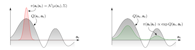
  传统的RL方法一般action是一个单峰的策略分布(unimodal policy distribution，下图中左图所示)，而我们想要探索整个的action分布，很自然的想法就是对其取幂，就变成了一个多峰策略分布 (multimodal policy distribution)。

• Energy based model和soft Q function的关系：

  由此作者使用了一种energy-based的policy方法，如下形式：

$$\pi \left({\mathbf{a}}_t|{\mathbf{s}}_t\right)\propto \exp \left(-\mathcal{E}\left({\mathbf{s}}_t,{\mathbf{a}}_t\right)\right)$$

  其中$\mathcal{E}$是energy function，可以用neural network来表示。

Theorem1. Let the soft Q-function be defined ：

  定义soft q function：

$$\begin{array}{l}{Q}_{\mathrm{s}\mathrm{o}\mathrm{f}\mathrm{t}}^{\ast }\left({\mathbf{s}}_t,{\mathbf{a}}_t\right)=r_t+\\ {\mathbb{E}}_{\left({\mathbf{s}}_{t+1},\dots \right)\sim {\rho }_{\pi }}\left[{\sum }_{l=1}^{\infty }{\gamma }^l\left(r_{t+l}+\alpha \mathcal{H}\left({\pi }_{\mathrm{M}\mathrm{a}\mathrm{x}\mathrm{E}\mathrm{n}\mathrm{t}}^{\ast }\left(\cdot |{\mathbf{s}}_{t+l}\right)\right)\right)\right]\end{array}$$

  和soft value function：

$$V_{\mathrm{s}\mathrm{o}\mathrm{f}\mathrm{t}}^{\ast }\left({\mathbf{s}}_t\right)=\alpha \log {\int }_{\mathcal{A}}\exp \left(\frac{1}{\alpha }{Q}_{\mathrm{s}\mathrm{o}\mathrm{f}\mathrm{t}}^{\ast }\left({\mathbf{s}}_t,{\mathbf{a}}^{\prime }\right)\right)d{\mathbf{a}}^{\prime }$$

  Maximum entropy RL算法的优化目标：

$${\pi }_{\mathrm{M}\mathrm{a}\mathrm{x}\mathrm{E}\mathrm{n}\mathrm{t}}^{\ast }=\arg \underset{\pi }{\max }\sum _t{\mathbb{E}}_{\left({\mathbf{s}}_t,{\mathbf{a}}_t\right)\sim {\rho }_{\pi }}\left[r\left({\mathbf{s}}_t,{\mathbf{a}}_t\right)+\alpha \mathcal{H}\left(\pi \left(\cdot |{\mathbf{s}}_t\right)\right)\right]$$

  由此可以得到上述Maximum entropy RL算法的优化目标的 the optimal policy：

$${\pi }_{\mathrm{M}\mathrm{a}\mathrm{x}\mathrm{E}\mathrm{n}\mathrm{t}}^{\ast }\left({\mathbf{a}}_t|{\mathbf{s}}_t\right)=\exp \left(\frac{1}{\alpha }\left(Q_{\mathrm{s}\mathrm{o}\mathrm{f}\mathrm{t}}^{\ast }\left({\mathbf{s}}_t,{\mathbf{a}}_t\right)-V_{\mathrm{s}\mathrm{o}\mathrm{f}\mathrm{t}}^{\ast }\left({\mathbf{s}}_t\right)\right)\right)$$

  Soft Q Learning中Policy Improvement 证明中有上述公式定义的部分解释(最优策略一定会满足这种energy-based的形式)。

  Theorem1将maximum entropy objective和energy-based的方法联系在一起了。其中$\frac{1}{\alpha }{Q}_{\mathrm{s}\mathrm{o}\mathrm{f}\mathrm{t}}\left({\mathbf{s}}_t,{\mathbf{a}}_t\right)$ acts as the negative energy。$\frac{1}{\alpha }{V}_{soft}(s_t)$ serve as the log-partition function。

Soft Q function会满足Soft Bellman Equation

$$Q_{\mathrm{s}\mathrm{o}\mathrm{f}\mathrm{t}}^{\ast }\left({\mathbf{s}}_t,{\mathbf{a}}_t\right)=r_t+\gamma {\mathbb{E}}_{{\mathbf{s}}_{t+1}\sim p_{\mathbf{s}}}\left[V_{\mathrm{s}\mathrm{o}\mathrm{f}\mathrm{t}}^{\ast }\left({\mathbf{s}}_{t+1}\right)\right]$$

  到此一些基本的定义就定义完成了，之后我们需要将Q-Learning的算法用于maximum entropy policy就可以了。

Training Expressive Energy-Based Models via Soft Q-Learning

  通过压缩映射能够证明：

$$\begin{array}{rl}{Q}_{\mathrm{s}\mathrm{o}\mathrm{f}\mathrm{t}}\left({\mathbf{s}}_t,{\mathbf{a}}_t\right)& \leftarrow r_t+\gamma {\mathbb{E}}_{{\mathbf{s}}_{t+1}\sim p_{\mathrm{s}}}\left[V_{\mathrm{s}\mathrm{o}\mathrm{f}\mathrm{t}}\left({\mathbf{s}}_{t+1}\right)\right],\forall {\mathbf{s}}_t,{\mathbf{a}}_t\\ V_{\mathrm{s}\mathrm{o}\mathrm{f}\mathrm{t}}\left({\mathbf{s}}_t\right)& \leftarrow \alpha \log {\int }_{\mathcal{A}}\exp \left(\frac{1}{\alpha }{Q}_{\mathrm{s}\mathrm{o}\mathrm{f}\mathrm{t}}\left({\mathbf{s}}_t,{\mathbf{a}}^{\prime }\right)\right)d{\mathbf{a}}^{\prime },\forall {\mathbf{s}}_t\end{array}$$

  会收敛到$Q_{soft}^{\ast }$和$V_{soft}^{\ast }$。然后这里还是有几个点需要去考虑，比如如何将其用于大规模的state、action空间。从energy-based中采样会变得很棘手(intractable)。

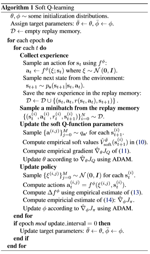
Soft Q Learning

  即使证明了soft贝尔曼方程会收敛，但是$V_{soft}^{\ast }$的计算过程中含有积分项，因此处理起来还是会很困难。作者用function approximator来定义$Q_{soft}^{\theta }(s,a)$。

  First，想要用stochastic optimization方法来对上述公式进行优化，我们首先将soft value function通过重要性采样得到其期望的形式：

$$V_{\mathrm{s}\mathrm{o}\mathrm{f}\mathrm{t}}^{\theta }\left({\mathbf{s}}_t\right)=\alpha \log {\mathbb{E}}_{q_{{\mathbf{a}}^{\prime }}}\left[\frac{\exp \left(\frac{1}{\alpha }{Q}_{\mathrm{s}\mathrm{o}\mathrm{f}\mathrm{t}}^{\theta }\left({\mathbf{s}}_t,{\mathbf{a}}^{\prime }\right)\right)}{q_{{\mathbf{a}}^{\prime }}\left({\mathbf{a}}^{\prime }\right)}\right]$$

  其中$q_{a^{\prime }}$可以为action space中的任意一个分布。我们可以将soft Q-Iteration 表示为最小化形式：

$$J_Q(\theta )={\mathbb{E}}_{{\mathbf{s}}_t\sim q_{s_t},{\mathbf{a}}_t\sim q_{{\mathbf{a}}_t}}\left[\frac{1}{2}{\left({\hat{Q}}_{\mathrm{s}\mathrm{o}\mathrm{f}\mathrm{t}}^{\bar{\theta }}\left({\mathbf{s}}_t,{\mathbf{a}}_t\right)-Q_{\mathrm{s}\mathrm{o}\mathrm{f}\mathrm{t}}^{\theta }\left({\mathbf{s}}_t,{\mathbf{a}}_t\right)\right)}^2\right]$$

  其中${\hat{Q}}_{\mathrm{s}\mathrm{o}\mathrm{f}\mathrm{t}}^{\bar{\theta }}\left({\mathbf{s}}_t,{\mathbf{a}}_t\right)=r_t+\gamma {\mathbb{E}}_{{\mathbf{s}}_{t+1}\sim p_{\mathbf{s}}}\left[V_{\mathrm{s}\mathrm{o}\mathrm{f}\mathrm{t}}^{\theta }\left({\mathbf{s}}_{t+1}\right)\right]$是target Q-Value。

Approximate Sampling and Stein Variational Gradient Descent (SVGD)

  那我们如何从soft q function中采样呢？传统的从energy-based分布中采样通常会有两种策略：1. use Markov chain Monte Carlo (MCMC) based sampling；2. learn a stochastic sampling network trained to output approximate samples from the target distribution . 然而作者依据2016年Liu, Q. and Wang, D.提出的两种方法，a sampling network based on Stein variational gradient descent (SVGD) 和 amortized SVGD.做采样。

• Liu, Q. and Wang, D. Stein variational gradient descent: A general purpose bayesian inference algorithm. In Advances In Neural Information Processing Systems, pp. 2370–2378, 2016.
• Wang, D. and Liu, Q. Learning to draw samples: With application to amortized mle for generative adversarial learning. arXiv preprint arXiv:1611.01722, 2016.

  这样做的好处主要有三点，提供一个stochastic sample generation；会收敛到EBM精确的后验分布；第三他可以跟actor critic算法联系起来，也就有了之后的SAC。

  我们想要去学习一个state-conditioned stochastic neural network ${\mathbf{a}}_t=f^{\varphi }\left(\xi ;{\mathbf{s}}_t\right)$，$\varphi$ 为网络参数，$\xi$ 为高斯或者其他任意一个分布的噪声。想要去寻找一个参数$\varphi$下的动作分布${\pi }^{\varphi }(a_t,s_t)$，期望这个分布能够近似energy-based的分布，KL divergence定义如下：

$$J_{\pi }\left(\varphi ;{\mathbf{s}}_t\right)=D_{KL}\left({\pi }^{\varphi }\left(\cdot |{\mathbf{s}}_t\right)\Vert \exp \left(\frac{1}{\alpha }\left(Q_{\text{soft }}^{\theta }\left({\mathbf{s}}_t,\cdot \right)-V_{\text{soft }}^{\theta }\right)\right)\right)$$

  Stein variationa lgradient descent如下：

$$\begin{array}{r}\Delta f^{\varphi }\left(\cdot ;{\mathbf{s}}_t\right)={\mathbb{E}}_{{\mathbf{a}}_t\sim {\pi }^{\varphi }}[\kappa \left({\mathbf{a}}_t,f^{\varphi }\left(\cdot ;{\mathbf{s}}_t\right)\right){\nabla }_{{\mathbf{a}}^{\prime }}]Q_{\mathrm{s}\mathrm{o}\mathrm{f}\mathrm{t}}^{\theta }\left({\mathbf{s}}_t,{\mathbf{a}}^{\prime }\right){|}_{{\mathbf{a}}^{\prime }={\mathbf{a}}_t}\\ +\alpha {\nabla }_{{\mathbf{a}}^{\prime }}\kappa ({\mathbf{a}}^{\prime },f^{\varphi }(\cdot ;{\mathbf{s}}_t)){|}_{{\mathbf{a}}^{\prime }={\mathbf{a}}_t}]\end{array}$$

  其中$\kappa$表示核函数，$\Delta f^{\varphi }$是the optimal direction of the reproducing kernel Hilbert space of $\kappa$，使用链导法则和Stein variational gradient into policy network我们有：

$$\frac{\partial J_{\pi }\left(\varphi ;{\mathbf{s}}_t\right)}{\partial \varphi }\propto {\mathbb{E}}_{\xi }\left[\Delta f^{\varphi }\left(\xi ;{\mathbf{s}}_t\right)\frac{\partial f^{\varphi }\left(\xi ;{\mathbf{s}}_t\right)}{\partial \varphi }\right]$$

取得的效果？

所出版信息？作者信息？

  这篇文章是ICML2017上面的一篇文章。第一作者Tuomas Haarnoja是Google DeepMind的research Scientist。

参考链接

• https://zhuanlan.zhihu.com/p/70360272

• https://zh.wikipedia.org/wiki/%E7%8E%BB%E5%B0%94%E5%85%B9%E6%9B%BC%E5%88%86%E5%B8%83

• https://zhuanlan.zhihu.com/p/44783057

• https://zhuanlan.zhihu.com/p/76681229

• https://www.dazhuanlan.com/2019/11/30/5de17e0ec54b1/

• 代码链接：https://github.com/haarnoja

扩展阅读

为什么要使用Stochastic Policy

  在有些情况下我们需要去学习一个stochastic policy，为什么要去学这样一个stochastic policy呢？作者举例了两点理由：

1. exploration in the presence of multimodal objectives(多模态的信息来源), and compositionality attained via pretraining. (Daniel et al., 2012)
2. 增加在不确定环境下的鲁棒性(Ziebart,2010)，在模仿学习中(Ziebartetal.,2008)，改善收敛性和计算性能( improved convergence and computational properties) (Gu et al., 2016a)

• 参考文献1：Daniel, C., Neumann, G., and Peters, J. Hierarchical relative entropy policy search. In AISTATS, pp. 273–281, 2012.
• 参考文献2：Ziebart,B.D. Modeling purposeful adaptive behavior with the principle of maximum causal entropy. PhD thesis, 2010.
• 参考文献3：Ziebart, B. D., Maas, A. L., Bagnell, J. A., and Dey, A. K. Maximum entropy inverse reinforcement learning. In AAAI Conference on Artificial Intelligence, pp. 1433– 1438, 2008.
• 参考文献4：Gu, S., Lillicrap, T., Ghahramani, Z., Turner, R. E., and Levine,S. Q-prop: Sample-efficientpolicygradientwith an off-policy critic. arXiv preprint arXiv:1611.02247, 2016a.

前人在 maximum entropy stochastic policy上的研究

1. Z-learning (Todorov, 2007)；

  Todorov, E. Linearly-solvable Markov decision problems. In Advances in Neural Information Processing Systems, pp. 1369–1376. MIT Press, 2007.

2. maximum entropy inverse RL(Ziebartetal.,2008)；

   Ziebart, B. D., Maas, A. L., Bagnell, J. A., and Dey, A. K. Maximum entropy inverse reinforcement learning. In AAAI Conference on Artificial Intelligence, pp. 1433– 1438, 2008.

3. approximate inference using message passing (Toussaint, 2009)；

• Toussaint, M. Robot trajectory optimization using approximate inference. In Int. Conf. on Machine Learning, pp. 1049–1056. ACM, 2009.

4. $\Psi$-learning (Rawlik et al., 2012)；

  Rawlik, K., Toussaint, M., and Vijayakumar, S. On stochastic optimal control and reinforcement learning by approximate inference. Proceedings of Robotics: Science and Systems VIII, 2012.

5. G-learning (Fox et al., 2016),

   Fox, R., Pakman, A., and Tishby, N. Taming the noise in reinforcement learning via soft updates. In Conf. on Uncertainty in Artificial Intelligence, 2016.

6. PGQ (O’Donoghue et al., 2016)；recent proposals in deep RL

   O’Donoghue, B., Munos, R., Kavukcuoglu, K., and Mnih, V. PGQ: Combining policy gradient and Q-learning. arXiv preprint arXiv:1611.01626, 2016

我的微信公众号名称：深度学习与先进智能决策
微信公众号ID：MultiAgent1024
公众号介绍：主要研究分享深度学习、机器博弈、强化学习等相关内容！期待您的关注，欢迎一起学习交流进步！

最后

以上就是优雅面包最近收集整理的关于【5分钟 Paper】Reinforcement Learning with Deep Energy-Based Policies的全部内容，更多相关【5分钟内容请搜索靠谱客的其他文章。