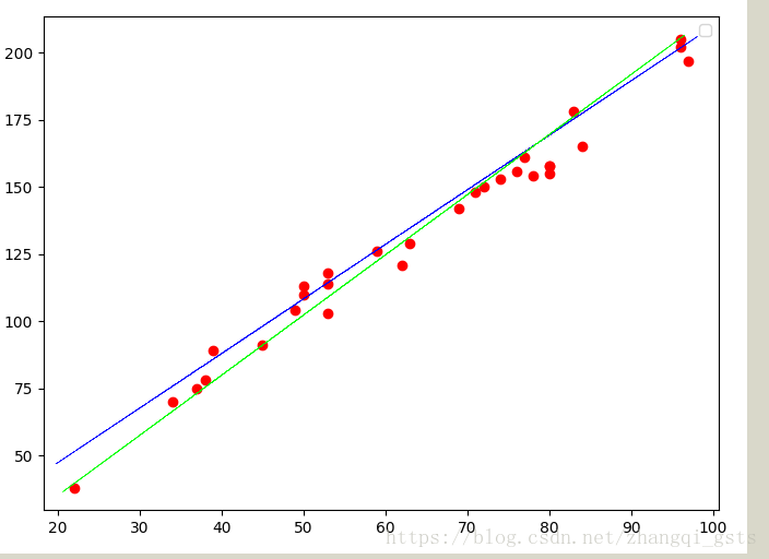
线性回归,我们在初中就开始接触了,二维平面给出一些点,用一条直线拟合这些点。但实际情况下,这些点中都会有一些噪点、误差,那么怎么才能找出一条拟合度最好的直线呢?比如下图是y=2x+4的点,随机加入一些误差后怎么才能得到拟合最好的直线。
要判断好还是不好,首先要有一个度量指标,其次这个指标可以容易转换成数学运算。这里引出一种方法:最小二乘法。 最小二乘的思路步骤如下: 1. 假设拟合直线为y=ax+b。2.对任意一点。3. 误差表示为
。4. 当
最小时拟合度最好。简单说,最小二乘法计算的是y的拟合值与实际值的差平方,而不是点
到直线的垂直距离,主要是因为计算点到直线的距离计算量比较复杂,而且也没必要。
知道了拟合好坏的衡量标准,那么机器学习的目的就是不断优化减小这个值。
#!/usr/bin/python
#encoding=utf-8
import tensorflow as tf
import numpy as np
import matplotlib.pyplot as plt
learn_rate = 0.01
#y=2x+4
#随机生成y=2x+4的一些坐标点
train_X = [np.random.randint(20, high=100) for x in range(30)]
train_Y = [2*x+4+np.random.randint(-10, high=10) for x in train_X]
#转成成numpy数组
train_X = np.array(train_X)
train_Y = np.array(train_Y)
n_samples = train_X.shape[0]
#用placeholder定义X和Y变量,具体值在训练的是用feed_dict填充
X = tf.placeholder(tf.float32)
Y = tf.placeholder(tf.float32)
#定义初始化W和b,一般不建议置0,用随机值初始化
W = tf.Variable(np.random.random(), name="weigth")
b = tf.Variable(np.random.random(), name="bias")
#带预测的线性方程
prediction = tf.add(tf.multiply(X, W), b)
#用最小二乘定义损失函数
cost = tf.reduce_mean(tf.square(prediction - Y))
#这里优化器并没有用梯度下降,而用的是Adam优化器,后面说明,优化,使得cost最小
#optimizer = tf.train.GradientDescentOptimizer(learn_rate).minimize(cost)
optimizer = tf.train.AdamOptimizer(learn_rate).minimize(cost)
init = tf.global_variables_initializer()
with tf.Session() as sess:
sess.run(init)
for i in range(1000):
for (x, y) in zip(train_X, train_Y):
#执行定义的优化器,填充placeholder定义的变量
sess.run(optimizer, feed_dict={X:x, Y:y})
if i % 50 == 0:
#每隔50次打印一次cost,由于cost依赖X和Y,所以也需要用feed_dict填充
c = sess.run(cost, feed_dict={X: train_X, Y: train_Y})
print("Epoch:", '%04d' % i, "cost=", "{:.9f}".format(c), "W=", sess.run(W), "b=", sess.run(b))
print("Optimization Finished!")
training_cost = sess.run(cost, feed_dict={X: train_X, Y: train_Y})
print("Training cost=", training_cost, "W=", sess.run(W), "b=", sess.run(b))
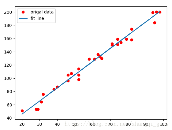
plt.plot(train_X, train_Y, 'ro', label="origal data")
plt.plot(train_X, sess.run(W) * train_X + sess.run(b), label="fit line")
plt.legend()
plt.show()
执行结果如下:
Epoch: 0000 cost= 4224.109863281 W= 1.0521932 b= 1.1191503
Epoch: 0050 cost= 36.584716797 W= 2.037287 b= 2.5342977
Epoch: 0100 cost= 36.166492462 W= 2.029028 b= 3.1004112
Epoch: 0150 cost= 35.803798676 W= 2.0202172 b= 3.6987798
Epoch: 0200 cost= 35.565029144 W= 2.0129821 b= 4.196062
Epoch: 0250 cost= 35.420043945 W= 2.0074644 b= 4.5785236
Epoch: 0300 cost= 35.332836151 W= 2.0033123 b= 4.8672404
Epoch: 0350 cost= 35.279922485 W= 2.0001948 b= 5.0842767
Epoch: 0400 cost= 35.247253418 W= 1.9978536 b= 5.247259
Epoch: 0450 cost= 35.226734161 W= 1.9960959 b= 5.3696275
Epoch: 0500 cost= 35.213581085 W= 1.9947772 b= 5.4614873
Epoch: 0550 cost= 35.204982758 W= 1.9937861 b= 5.5304694
Epoch: 0600 cost= 35.199237823 W= 1.9930426 b= 5.5822573
Epoch: 0650 cost= 35.195346832 W= 1.9924846 b= 5.6211405
Epoch: 0700 cost= 35.192630768 W= 1.9920651 b= 5.650337
Epoch: 0750 cost= 35.190742493 W= 1.9917507 b= 5.672256
Epoch: 0800 cost= 35.189373016 W= 1.9915143 b= 5.688697
Epoch: 0850 cost= 35.188400269 W= 1.9913368 b= 5.7010508
Epoch: 0900 cost= 35.187698364 W= 1.9912037 b= 5.710329
Epoch: 0950 cost= 35.187175751 W= 1.9911035 b= 5.717318
Optimization Finished!
Training cost= 35.186806 W= 1.9910296 b= 5.7224526
最后得到W是1.9,b是5.7,由于加入了噪点,所以b比实际的y=2x+4中的4偏大
注意上面,在定义优化器的时候并没有用梯度下降,因为在用梯度下降的时候训练几次就会出现nan。
Epoch: 0000 cost= inf W= -9.956399e+27 b= -1.1271411e+26
Epoch: 0001 cost= nan W= nan b= nan
Epoch: 0002 cost= nan W= nan b= nan原因是设置学习速率太快了,很快就溢出。解决办法有两种,一种是不用梯度下降,而采用Adam,另一种办法是不将损失函数的最小二乘法做一下修改,改成cost = tf.reduce_sum(tf.pow(prediction-Y, 2) / (2*n_samples))
最后
以上就是迷人小天鹅最近收集整理的关于TensorFlow基础之线性回归的全部内容,更多相关TensorFlow基础之线性回归内容请搜索靠谱客的其他文章。
本图文内容来源于网友提供,作为学习参考使用,或来自网络收集整理,版权属于原作者所有。


发表评论 取消回复